Here is a next-step analysis jumping off of the web scraping and mapping post from a couple of months back. Showing points on a map is great for big picture visualizations, but what if we need to know a little more? Maybe we’re interested in relationships between points. Or specifically, how far are these point from each other? We can calculate euclidean distances between our points, but this doesn’t really translate to the real world. On a map, no 2 distances are ever really equal. For example, it takes about 30 minutes to drive from the Inwood, the most northern neighborhood in Manhattan, to Battery Park in the south. In the same amount of time it takes to cover those 13 miles in NYC, one can cover about double the distance driving from Grand Rapids to the city of Holland in Western Michigan.
With my mapping project, we needed a way to classify points based on their driving distance from a group of key addresses, which were already existing outdoor specialty accounts. We wanted to expand distribution with as little effect on our already established core business partners. I came across the gmapdistance package, developed and maintained by economist Rodrigo Azuero. There were 3 big appeals for me -
- It returns a list of 3 values: status of the query, driving distance in meters, and driving time in seconds.
- It can run on 2 vectors of locations, returning a list of matrices covering each combination of inputs.
- It takes longitude and latitude as inputs, which we’ve already retrieved in the last exercise.
With my vectors of scraped Dillard’s stores and outdoor specialty locations, I set out to find an optimal group for expansion.
Setup
To get started, we need the below libraries.
library(tidyverse)
library(ggmap)
library(gmapsdistance)
library(knitr)
Similar to the the coordinate retriever, we will need to set up our Google Maps API key. You can use this video to guide you through set up. The set.api.key sort of applies our key to the environment, allowing us to call the API without having to specify it each time.
google_api_key <- "your_key"
register_google(key = google_api_key)
set.api.key(google_api_key)
Data Collection
Because this was covered in this post, I will simply load in my addresses. This can be done with any vector of addresses. They don’t even need to be in the formal street-city-state-postal format either! Anything that you’d search for in Google Maps will function.
The gmapdistance Package
The main function in this package is gmapdistance. It needs 3 minimum arguments: origin, destination, and mode. The last of which takes “bicycling”, “walking”, “transit”, or “driving” as a string. Note that we need to use + anywhere we’d have a space.
gmapsdistance(origin = "inwood+manhattan",
              destination = "battery+park",
              mode = "driving")
## $Time
## [1] 1882
##
## $Distance
## [1] 20896
##
## $Status
## [1] "OK"The function returns a named list of length 3:
- Time - number of seconds to complete the specified trip.
- Distance - number of meters for the specified trip.
- Status - returns “OK” if retrieval did not cause an error.
So, it takes about 30 minutes (1803 seconds / 60) to go from the Inwood neighborhood to Battery Park in Manhattan. Let’s check Grand Rapids to Holland, MI!
gmapsdistance(origin = "grand+rapids+mi",
              destination = "holland+mi",
              mode = "driving")
## $Time
## [1] 2336
##
## $Distance
## [1] 52443
##
## $Status
## [1] "OK"Almost the same amount of time driving, yet we cover so much more ground! These sets of points are proving to be similar in terms of proximity - something we wold not have discovered using euclidean distance.
Vector Inputs
The real power of this function comes in its ability to work with vectors of locations.
origins <- c("inwood+manhattan", "grand+rapids+mi", "washington+memorial")
destinations <- c("battery+park+ny", "holland+mi", "white+house+dc")

vector_inputs <- gmapsdistance(origin = origins,
                               destination = destinations,
                               mode = "driving")

vector_inputs$Time %>% kable()| or | Time.battery+park+ny | Time.holland+mi | Time.white+house+dc |
|---|---|---|---|
| inwood+manhattan | 1882 | 42383 | 14337 |
| grand+rapids+mi | 40724 | 2336 | 35732 |
| washington+memorial | 13608 | 36996 | 310 |
Similarly, the function returns a list of length 3, but each entry is a data frame with dimensions dependent on the input vectors. Looking at the times above, we see the ~30 minute trips from Inwood to Battery Park and Grand Rapids to Holland, while the Washington Memorial is just 5 minutes from the White House.
Processing Considerations
In the above example, we see that 9 trips were retrieved from the API. Each of these takes time and a long vector can make a script cumbersome. See below run time using system.time:
system.time({gmapsdistance(origin = origins,
                           destination = destinations,
                           mode = "driving")})
## user system elapsed
## 0.28 0.00 10.72Run time hovers around 10 - 12 seconds. From my experience, a retrieval will be timed at about 1 second a piece. It’s important to hone in on your interested list before running any vectors of locations. There is a combinations argument that will compute either all combinations (“all”) or just corresponding entries (“pairwise”). This is useful if you’ve got specific pairs of locations you want to investigate.
Other Arguments for Tuning
The function has additional default arguments that can be modified including traffic_model (“optimistic” vs “pessimistic”), avoid (“tolls”, “highways”), and even arrival or departure times.
Using Longitude and Latitude as Inputs
Because I was storing longitude and latitude features in order to plot the locations on a map, I used another useful feature of the gmapdistance function - it takes coordinates, too! Specifically in “lat+lon” format. Using our sample vectors:
origins %>%
  data_frame(locations = .) %>%
  mutate_geocode(locations) %>%
  mutate(dist_input = paste0(lat, "+", lon)) %>%
  kable()
## Warning: `data_frame()` is deprecated, use `tibble()`.
## This warning is displayed once per session.| locations | lon | lat | dist_input |
|---|---|---|---|
| inwood+manhattan | -73.92120 | 40.86771 | 40.8677145+-73.9212019 |
| grand+rapids+mi | -85.66809 | 42.96336 | 42.9633599+-85.6680863 |
| washington+memorial | -77.03528 | 38.88948 | 38.8894838+-77.0352791 |
destinations %>%
  data_frame(locations = .) %>%
  mutate_geocode(locations) %>%
  mutate(dist_input = paste0(lat, "+", lon)) %>%
kable()| locations | lon | lat | dist_input |
|---|---|---|---|
| battery+park+ny | -74.01703 | 40.70328 | 40.7032775+-74.0170279 |
| holland+mi | -86.10893 | 42.78752 | 42.7875235+-86.1089301 |
| white+house+dc | -77.03653 | 38.89768 | 38.8976763+-77.0365298 |
The dist_input column is now ready to be used as an input to gmapdistance!
Finding the best Dillards
The above method was used to convert the lists of potential Dillards locations and current Outdoor Specialty accounts into 2 input vectors in the dist_input format. As mentioned above, the vectors of just a few hundred entries would have produced a massive data frame of retrievals. To cut back on run time, I prefiltered the vectors based on state and then ran them through the gmapdistance function. Below sample was used to build a function that applied to a list of states.
# Prefilter both groups to cut on processing
dillards_fl <- dillards_dist %>% filter(state == "FL")
outdoor_fl <- outdoor_dist %>% filter(state == "FL")

# Run function
output_fl <- gmapsdistance(dillards_fl$dist_input, outdoor_fl$dist_input, mode = "driving")

# Add address field to line up coordinate inputs with readable locations
output_fl$Time <- dillards_fl$address

# Store time only
time_matrix_fl <- output_fl$Time

# Function
get_distances <- function(..state, group_1, group_2){
  group_1_filt <- group_1 %>% filter(state == ..state)
  group_2_filt <- group_2 %>% filter(state == ..state)
  output <- gmapsdistance(group_1_filt$dist_input, group_2_filt$dist_input, mode = "driving")
  output$Time <- group_1_filt$address
  return(output$Time)
}
Using tidyr::gather to Analyze
The dataframe output is useful at a glance, but we are better off using a long table to systematically analyze. Using gather allows us to see the travel time for specific pairs of locations. For better readability, we can add in a column to show the time in minutes using mutate.
vector_inputs$Time %>%
  gather(destination, time, -or) %>%
  mutate(time_minutes = round(time / 60.0, digits = 0))
## or destination time time_minutes
## 1 inwood+manhattan Time.battery+park+ny 1882 31
## 2 grand+rapids+mi Time.battery+park+ny 40724 679
## 3 washington+memorial Time.battery+park+ny 13608 227
## 4 inwood+manhattan Time.holland+mi 42383 706
## 5 grand+rapids+mi Time.holland+mi 2336 39
## 6 washington+memorial Time.holland+mi 36996 617
## 7 inwood+manhattan Time.white+house+dc 14337 239
## 8 grand+rapids+mi Time.white+house+dc 35732 596
## 9 washington+memorial Time.white+house+dc 310 5Using various time thresholds, I was able to grade each individual Dillard’s location by how many Outdoor Specialty stores were within that many minutes of driving.
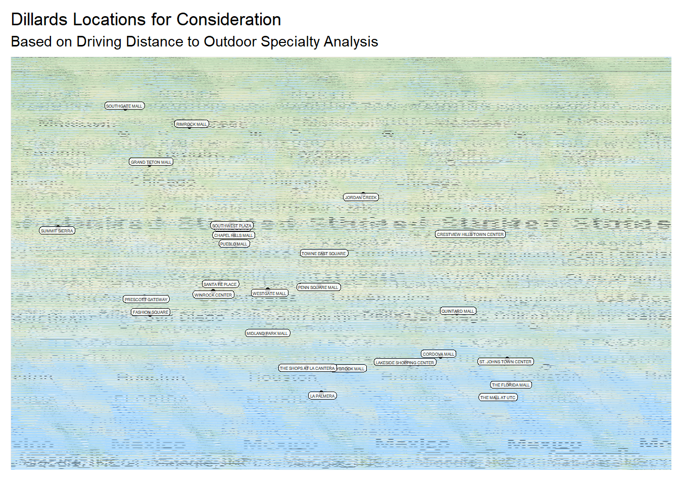
Final Map
After agreeing on driving time thresholds, the driving distances between pairs were filtered and counted against each Dillard location. For example, Store in Mall X has 2 outdoor specialty accounts within a 30 minute drive. Is that acceptable?
After internal discussions, we decided on a selection of stores and ran the below map showing mall names and locations to communicate with our partners.
# Plot malls on US map with labels showing mall name.
ggmap(mapped_region) +
  geom_point(aes(x = lon, y = lat), alpha = 0.8, data = final_list_coord) +
  geom_label(aes(x = lon, y = lat, label = Mall),
             position = position_jitter(width = 0.2, height = 0.2),
             label.padding = unit(0.1, "lines"),
             alpha = 0.8, size = 1, data = final_list_coord) +
  theme(axis.title = element_blank(),
        axis.text = element_blank(),
        axis.ticks = element_blank(),
        legend.position = "top",
        legend.title = element_blank()) +
  ggtitle(label = "Dillards Locations for Consideration",
          subtitle = "Based on Driving Distance to Outdoor Specialty Analysis")