Background

The Color + Trend team at Chaco designs every webbing placed on our Z sandals from a collection of threads. The very talented group puts together visually striking patterns that allow us to offer fresh takes on our classic silhouette annually.

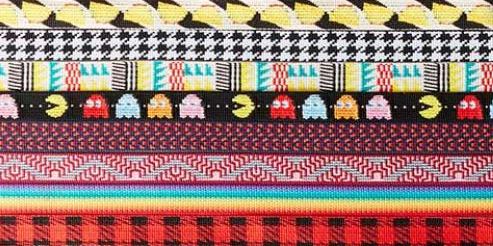
A few styles

It takes a lot of work and subsequently lots of PhotoShop, InDesign, and PDF files to get a collection of styles out the door and into the retail market.

When a season starts, the team generates a color palette to work with.

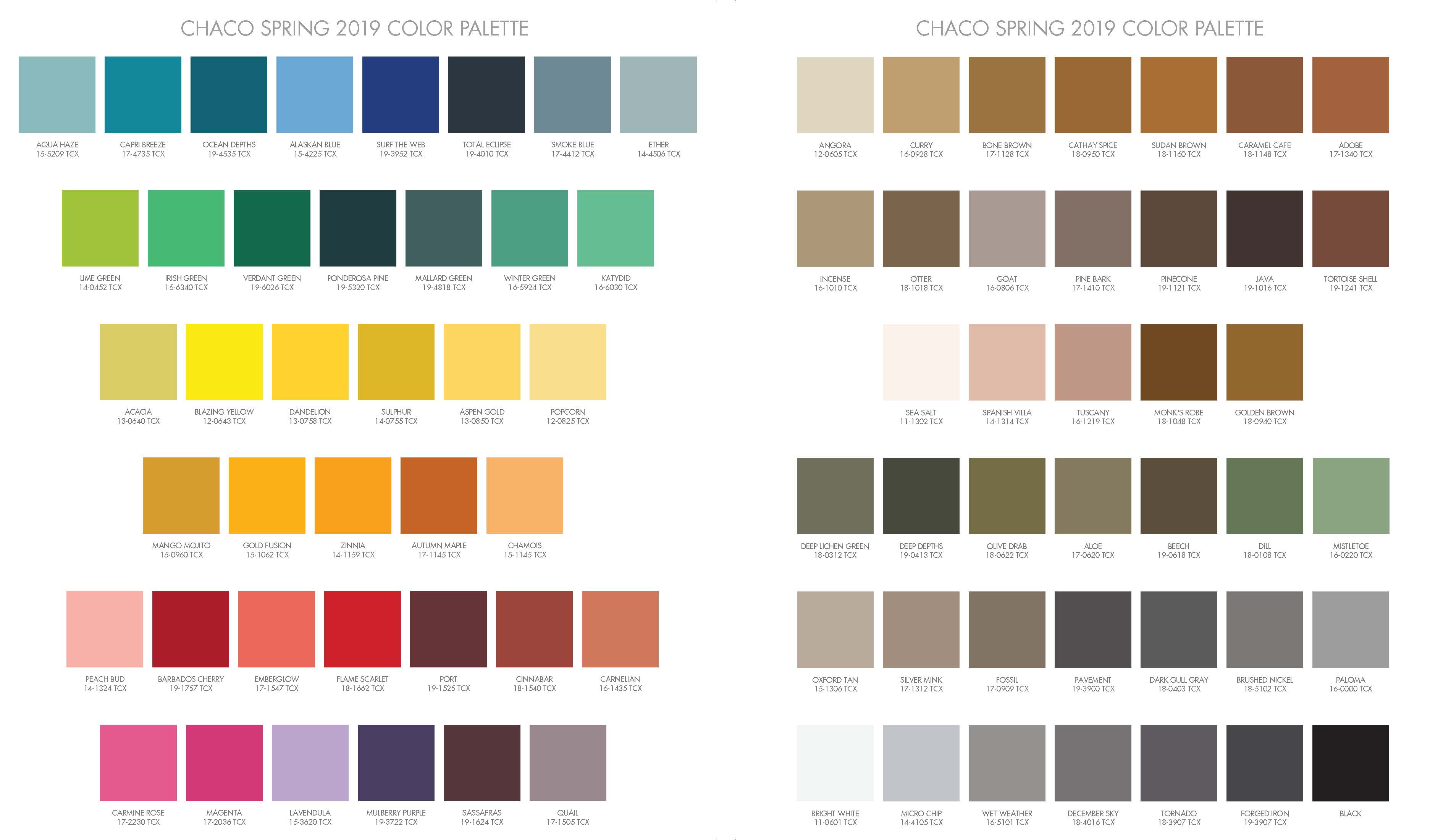
The blues, greens, reds, and grays are selected and placed into intricate patterns. The team makes hundreds at a time and widdles them down to a complete assortment. Through the design process, all of the yarns are used, but the downstream style may not pass review or be dropped from production.

This lead to a product manager reaching out to me with what started out as simple questions:

• what is the best way to see how often each yarn gets used?
• Can we find where each yarn is being used?
• Are there any yarns we are not using?

Data Exploration and Plan of Attack

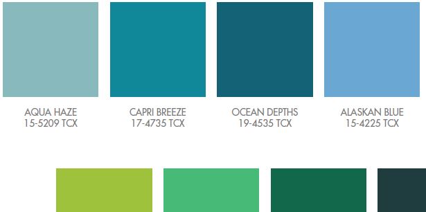
In the palette above, each of the squares represents a specific yarn or thread color that is to be woven into a style. Looking closer, I saw that each color had a unique code in the format ##-####:

When looking at the pdf files produced by the design team, I saw that each yarn color is included in their stored filed, outlined below in blue.

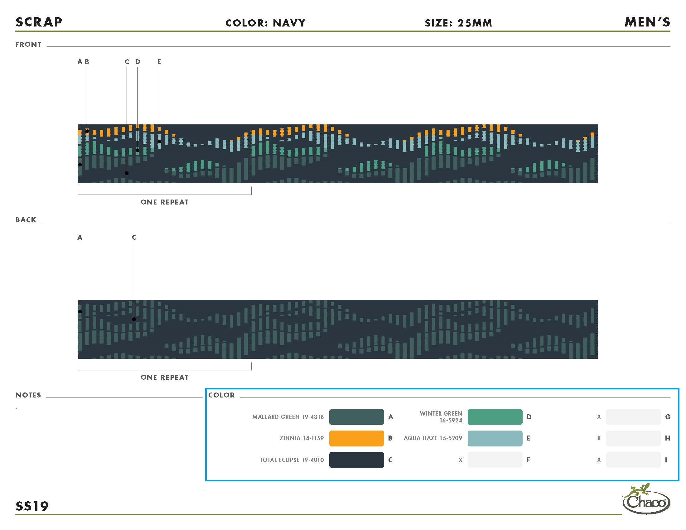
So, if I knew how to read the content on these PDF files and extract the color codes, I’d be able to link yarns to each file. I came across this Stack Overflow post. I followed the advice from Remko Duursma and tried out the pdftools package. Using its function pdf_text and some regular expression with stringr, I felt confident that I could extract the ##-#### patterns from an arbitrary file.

The next hurdle was to know where to find these files. I quickly learned that I am VERY fortunate for the meticulous file-folder naming scheme that the product team uses. Not only is there a logical hierarchy of folders that go from the selling season, through to gender, then to the pattern, but the color files also had season, gender, color, and webbing width consistently built in.

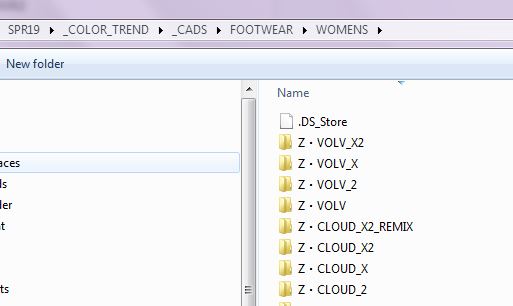
Great folders

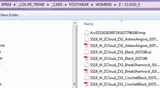
With even better file names

Now knowing the paths to all of the necessary files, along with the tools to collect the color codes within them, I set off to turn the directory of product files into a clean, succinct dataframe.

Before we dive into the nitty gritty - the Payoff

The below was a first look at how we were doing with yarn usage. You can see the top 3 yarns are used quite a bit more than number 4. There is also a tail of yarns that are only present in 1-2 patterns, with some coming in at no usage.

yarn %>%
  group_by(color_code, color_name) %>%
  summarize(style_count = sum(style_count)) %>%
  ggplot(aes(x = fct_reorder(color_name, -style_count), y = style_count)) +
    geom_col(fill = "darkgreen") +
    theme(axis.text.x = element_text(angle = 90, hjust = 1, vjust = 0, size = 5),
          axis.title.x = element_blank(),
          axis.title.y = element_blank(),
          axis.ticks.y = element_blank()) +
  ggtitle("Yarn Colors vs Times Represented in SPR19 Styles")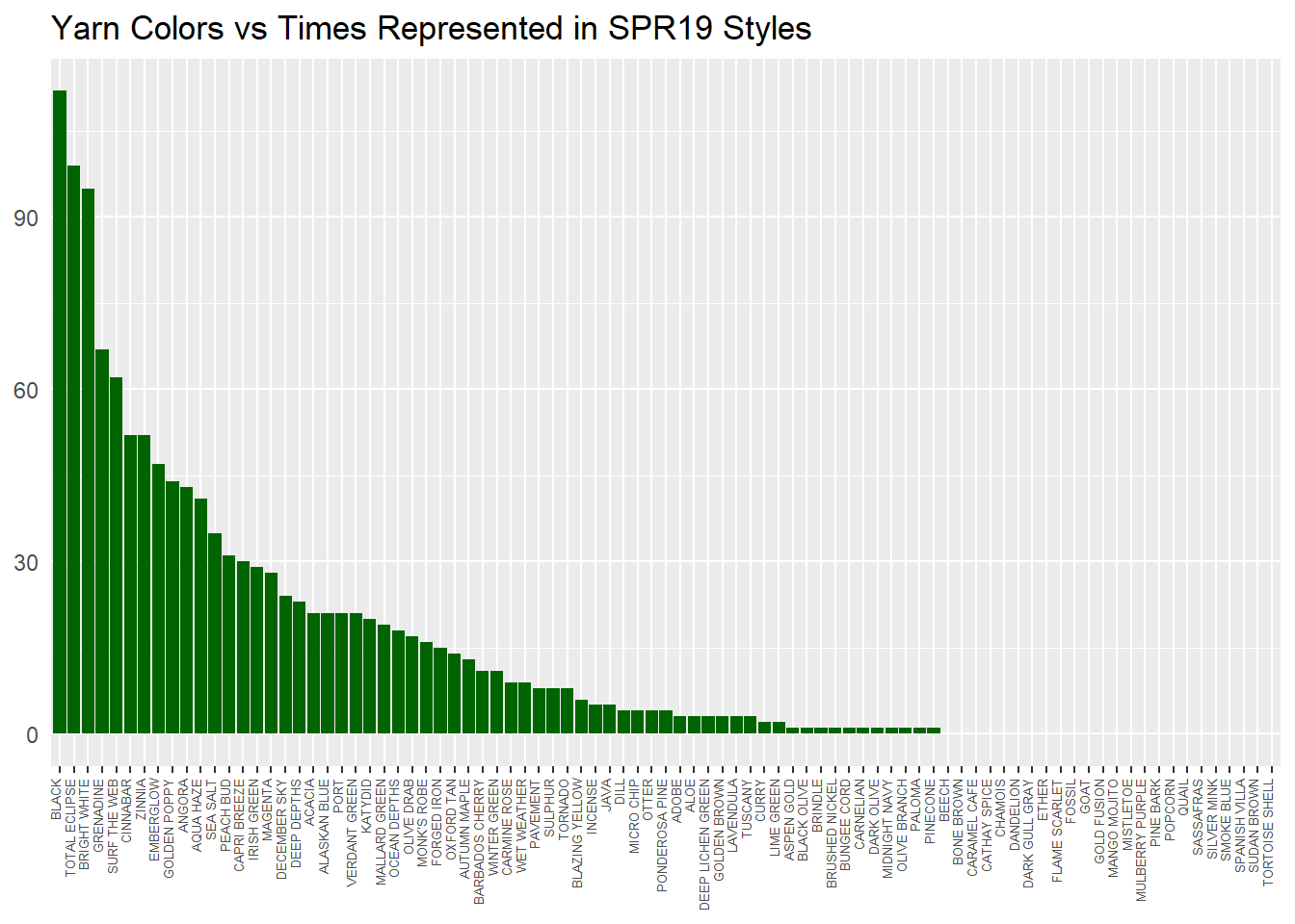

Keep scrolling for a technical dive into the process.

dir() Function

For footwear, there is typically a pattern or style which has a number of color options. For example, Chaco has the men’s Z1 Classic, a pattern that is available in the colors black, tri java, and split gray. The team groups the color files, of which we’re scanning for yarn, in folders named after the patterns. There are specific patterns in which webbing is used.

I initially thought I’d scan pdfs in each folder by hard keying the directory path to those files, but that was cumbersome and inefficient, especially if any new patterns were introduced. Looking for methods to find directories, I did some deeper research on the dir function in base R. From ?dir:

Description
These functions produce a character vector of the names of files or directories in the named directory.

Specifically, the full.names and pattern arguments were most helpful. On default, dir returns a character string of all folders and files.

dir("sample_folder/sample_subfolderA/sample_subfolderB")

## [1] "sample_file.txt"       "sample_file_CHACO.txt"

If we add the full.names = TRUE argument, we get an absolute path.

dir("sample_folder/sample_subfolderA/sample_subfolderB", full.names = TRUE)

## [1] "sample_folder/sample_subfolderA/sample_subfolderB/sample_file.txt"      
## [2] "sample_folder/sample_subfolderA/sample_subfolderB/sample_file_CHACO.txt"

Scanning folders for the needed pdfs with full.names = TRUE, we can pass an absolute path to pdf reader to scan for color codes AND classify the colors extracted by style, gender, and season. To pull only pdfs, we use the pattern argument, which accepts regex inputs.

dir("sample_folder/sample_subfolderA/sample_subfolderB", 
    full.names = TRUE, 
    pattern = "*_CHACO.txt")

## [1] "sample_folder/sample_subfolderA/sample_subfolderB/sample_file_CHACO.txt"

Building the Function

To make good use of my time, I built a group of functions to split out code responsibilities and make what I was doing readable. See the below snippets I needed to implement, followed by the functions that combined them.

Using dir, I passed the gender-level folder and scanned for folders with webbing-based patterns. The or() function from the rebus package makes the code super readable. If you’re working a lot in regex, I recommend rebus for ease.

directory <- dir(path = ..path,
                 pattern = or("CLASSIC", "CANYON", "CLOUD", "VOLV",
                              "BOULDER", "PLAYA", "LOVELAND", "MIA",
                              "1IN BELT", "BOB BELT", "DOG LEASH_COLLAR", "WRIST WRAP",
                              "DAY_PACK", "HIP_BAG", "SLING", "TOTE", "TEGU"),
                 full.names = TRUE)

With the absolute paths to all of the above folers, I implemented another dir layer to retrieve the paths to the actual files. I used map from the purrr package to apply the function to each subfolder. unlist converted the output list to character vector of paths to pdf files.

  full_file_list <- map(directory, dir, pattern = "*.pdf", full.names = TRUE) %>% unlist()

The full file names are useful for retrieving, but is cumbersome for our table. The following line replaces the path given with an empty string and stores it for later.

  list_names <- full_file_list %>% str_replace(paste0(..path, "/"), "")

At this point, we have a full vector of path names to a pdf with color codes within it. The next phase of coding needs to scan the file and extract the ##-#### format we discovered earlier. The pdftools::pdf_text function extracts all text from a pdf and stores it as a character vector of length one.

swatch <- pdf_text(paste0(..path))

Then we get to use rebus again. Since we are looking for any 2 digits, followed by a “-”, then followed by any 4 digits, we would traditionally use the regex [0-9]{2}-[0-9]{4}. The rebus package allows us to write this using readable functions and a pipeline syntax that is reminiscent of tidyverse’s %>%.

 ..list <- str_extract_all(swatch, pattern = 
                             ascii_digit(2,2) %R%
                             "-" %R%
                             ascii_digit(4,4)) 

The above produces a list of color code character vectors with the pdf name as each list element’s name. The last step here is to transform this into a dataframe. Below we use unlist twice - once to extract the list names into the column “pattern_color” and another to grab the character vector at each list entry. Since we extract the names under “pattern_color”, we can set use.names = FALSE in the second use.

  df <- data.frame("pattern_color" = names(unlist(..list)), 
                   "color_code" = unlist(..list, use.names = FALSE))

Then we do some processing - split the “pattern_color” column, take out “.pdf”, season, and gender tags. Again using rebus for regex support. Also included a new gender column that will be hard keyed in.

  df %>%
    separate(pattern_color, c("pattern", "color"), "/") %>%
    mutate(color = str_replace(color, ".pdf" %R% optional(DIGIT), ""),
           color = str_replace(color, START %R% alpha(2,2) %R% digit(2,2) %R% "_" %R% ALPHA %R% "_", ""),
           gender = "gender label")

While building the functions to facilitate these steps, I noticed an issue with black yarn. This color is used every year and so is not assigned a color code, causing it to not get picked up by the ##-#### scanner. To handle, I added in a get_black argument to the below functions that would search for BLACK instead of ##-#### if set to true. Then each folder would get scanned twice - once for black yarn and once for all others.

get_styles <- function(..path, get_black = FALSE){
  # Looks for all folders with the below patterns in the name
  directory <- dir(path = ..path, 
                   pattern = or("CLASSIC", "CANYON", "CLOUD", "VOLV", 
                                "BOULDER", "PLAYA", "LOVELAND", "MIA",
                                "1IN BELT", "BOB BELT", "DOG LEASH_COLLAR", "WRIST WRAP",
                                "DAY_PACK", "HIP_BAG", "SLING", "TOTE", "TEGU"), 
                   full.names = TRUE)
  
  # Runs through each folder and retrieves the name of all .pdf files. 
  full_file_list <- map(directory, dir, pattern = "*.pdf", full.names = TRUE) %>% unlist()
  
  # Remove absolute directory portion to have readable names for the yarn extracts
  list_names <- full_file_list %>% str_replace(paste0(..path, "/"), "")

  # get_black deciphers whether to look for ##-#### color code or "BLACK"
  if(get_black) listed <- full_file_list %>% 
    map(get_color_codes, get_black = TRUE) %>% 
    set_names(list_names)
  else listed <- full_file_list %>% 
    map(get_color_codes, get_black = FALSE) %>% 
    set_names(list_names)
  
  return(listed)
}

get_color_codes <- function(..pdf_path, get_black = FALSE){
  swatch <- pdf_text(paste0(..pdf_path))
  
  if(get_black){
    str_extract_all(swatch, "BLACK") %>%
      unlist()
  }
    
  else{
    # if not looking for black yarn, pull ##-####
    str_extract_all(swatch, ascii_digit(2,2) %R%
                      "-" %R%
                      ascii_digit(4,4)) %>%
      unlist()   
  }
}

list_to_df <- function(..list, ..gender){
  df <- data.frame("pattern_color" = names(unlist(..list)), 
                   "color_code" = unlist(..list, use.names = FALSE))
  
  df %>%
    separate(pattern_color, c("pattern", "color"), "/") %>%
    mutate(color = str_replace(color, ".pdf" %R% 
                                 optional(DIGIT), ""),
           color = str_replace(color, START %R% 
                                 alpha(2,2) %R% 
                                 digit(2,2) %R% 
                                 "_" %R% 
                                 ALPHA %R% 
                                 "_", ""),
           gender = ..gender)  
}

Sample pipeline for a single path

# set high level folder path
women_path <- "//wwwint.corp/dfs/ROC/ChacoPD/SPR19/_COLOR_TREND/_WEBBING/_LINE/FOOTWEAR/WOMENS"

# get individual file paths 
womens <- get_styles(women_path)
womens_black <- get_styles(women_path, get_black = TRUE)

# set as df
womens_df <- list_to_df(womens, "womens")
womens_black_df <- list_to_df(womens_black, "womens")

# combine into single df, use color code file as a lookup, factor pattern and gender
all_styles <- bind_rows(womens_df, womens_black_df) %>%
  left_join(code_lookup, by = c("color_code" = "Color Code")) %>%
  mutate(pattern = factor(pattern),
         gender = factor(gender))

# Write to .csv to be loaded in by markdown file. Full join color lookup here to include any colors not used.
all_styles %>%
  group_by(color_code, `Color Name`) %>%
  summarize(style_count = n()) %>%
  arrange(desc(style_count)) %>%
  full_join(code_lookup, by = c("color_code" = "Color Code")) %>%
  mutate(`Color Name.x` = if_else(is.na(`Color Name.x`), `Color Name.y`, `Color Name.x`),
         style_count = if_else(is.na(style_count), as.double(0), as.double(style_count))) %>%
  select(color_code, "color_name" = `Color Name.x`, style_count) %>%
  write_csv("Yarn Colors - Number of SPR19 Styles.csv")

Running the above for each gender folder, as well as special capsule folders that hold additional webbing styles, generates a total dataframe, cleaned for analysis.

The .csv file written on the last line below is what was plugged into the ggplot graph above.