Packages

• As mentioned above, rvest contains our web scraping functions.
• ggmap interfaces with the google API to produce maps that can be layered with data using ggplot from the tidyverse packages.
• The locations of the non-Dillards locations are stored in Excel files, so I’m including readxl.

library(rvest)
library(ggmap)
library(tidyverse)
library(readxl)

Scraping Dillard’s Locations

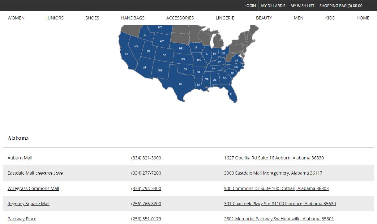
Luckily for us, Dillard’s store locator is SUPER web scraper friendly because all addresses are stored in a single line of text and are all shown on one page!

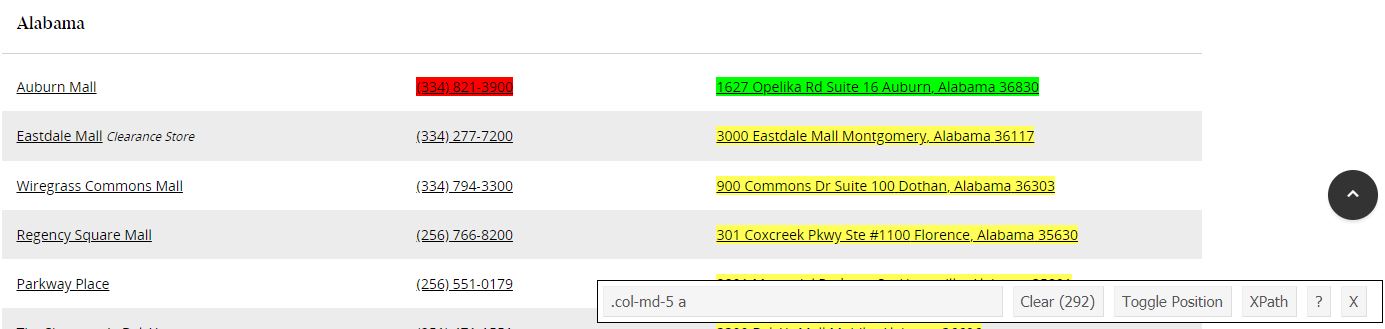
Using the Selector Gadget, we’re able to pinpoint which tag is associated with the full addresses. In this case, .col-md-5 a is what we’ll focus our scraper on.

So, using read_html with the location of the web page, html_nodes to focus on our tag, and html_text to retrieve the text that sits there, we’re able to scrape all addresses of Dillard’s Department stores in the US.

dillards <- read_html("https://www.dillards.com/stores") %>%
  html_nodes(".col-md-5 a") %>%
  html_text()

# Make into 1 column dataframe with a header
dillards <- data.frame("address" = dillards)

# See first 15 entries
head(dillards, n = 15)

##                                                  address
## 1            3000 Eastdale MallMontgomery, Alabama 36117
## 2                 3300 Bel Air MallMobile, Alabama 36606
## 3    10101 Eastern Shore BlvdSpanish Fort, Alabama 36527
## 4          1627 Opelika Rd Suite 16Auburn, Alabama 36830
## 5          900 Commons Dr Suite 100Dothan, Alabama 36303
## 6     301 Coxcreek Pkwy Ste #1100Florence, Alabama 35630
## 7      2801 Memorial Parkway SwHuntsville, Alabama 35801
## 8        7310 Eastchase ParkwayMontgomery, Alabama 36117
## 9                   700 Quintard DrOxford, Alabama 36203
## 10             1435 West Southern AveMesa, Arizona 85202
## 11        10002 Metro Parkway EastPhoenix, Arizona 85051
## 12        3101 West Chandler BlvdChandler, Arizona 85226
## 13     2151 S. San Tan Village PkyGilbert, Arizona 85296
## 14 7800 W. Arrowhead Towne CenterGlendale, Arizona 85308
## 15               6545 E. Southern AveMesa, Arizona 85206

Combining With Other Data

The two other stores’ locations are stored in 2 spreadsheets - one with full addresses in a single line and one with street number, city, state, and postal code in separate fields - the functions for retrieving coordinates can take a full string as an address, so we’ll want to process everything into a single columne dataframe. After reading these in with readxl, we combine everything using dplyr::bind_rows.

# Simple case, data in the format we need.
store_x <- read_excel("Store X list.xlsx", 
                      sheet = "store_list", 
                      col_names = c("address"), 
                      col_types = c("text"))

# This spreadsheet needs some processing, combining the columns into a single 
# column using mutate, then selecting that column.
store_y <- read_excel("Store Y list SS2018.xlsx", sheet = "store_list") %>%
  mutate(address = paste(Address, City, State, Zip)) %>%
  select(address)

# Combine our 3 data sources into one data frame.
all_stores <- bind_rows("Dillard's" = dillards, 
                        "Store X" = store_x, 
                        "Store Y" = store_y, 
                        .id = "retailer")

head(all_stores, n = 15)

##     retailer                                               address
## 1  Dillard's           3000 Eastdale MallMontgomery, Alabama 36117
## 2  Dillard's                3300 Bel Air MallMobile, Alabama 36606
## 3  Dillard's   10101 Eastern Shore BlvdSpanish Fort, Alabama 36527
## 4  Dillard's         1627 Opelika Rd Suite 16Auburn, Alabama 36830
## 5  Dillard's         900 Commons Dr Suite 100Dothan, Alabama 36303
## 6  Dillard's    301 Coxcreek Pkwy Ste #1100Florence, Alabama 35630
## 7  Dillard's     2801 Memorial Parkway SwHuntsville, Alabama 35801
## 8  Dillard's       7310 Eastchase ParkwayMontgomery, Alabama 36117
## 9  Dillard's                  700 Quintard DrOxford, Alabama 36203
## 10 Dillard's             1435 West Southern AveMesa, Arizona 85202
## 11 Dillard's        10002 Metro Parkway EastPhoenix, Arizona 85051
## 12 Dillard's        3101 West Chandler BlvdChandler, Arizona 85226
## 13 Dillard's     2151 S. San Tan Village PkyGilbert, Arizona 85296
## 14 Dillard's 7800 W. Arrowhead Towne CenterGlendale, Arizona 85308
## 15 Dillard's               6545 E. Southern AveMesa, Arizona 85206

Mapping Our Store Locations

Our next phase is to interface with the Google Maps API. Once we build a connection, we can retrieve a map of the US and the coordinates for each element of the address list we constructed above. As of Summer 2018, Google updated their pricing structure for their Maps API. You can use this video to guide you through setting up your key. Note you will be prompted to enter billing information, though if your usage is low enough - fewer than 2,500 queries a day - you won’t incur any charges.

So, we’ll first register our API using ggmap::register_google

google_api_key <- "your_key_here"
register_google(key = google_api_key)

Once we’re connected, we’ll want to grab a map of the US to layer onto using get_googlemap.

• The center argument can be anything you would type into Google Maps to find - “Grand River, MI” or “Statue of Liberty” or even an address.
• The zoom argument takes an integer argument ranging from 3 (continent) to 21 (a building). By default, a city is shown at level 10.
  
• size argument maxes out at 640 x 400.
• The function returns an object of type ggmap, which we can then look at using ggmap. Note that the x and y axis are represented as longitude and latitude, respectively. This is a key because we’ll have coordinates in this form for our store locations!

mapped_region <- get_googlemap(center = "united states", zoom = 4, size = c(640, 400))

ggmap(mapped_region)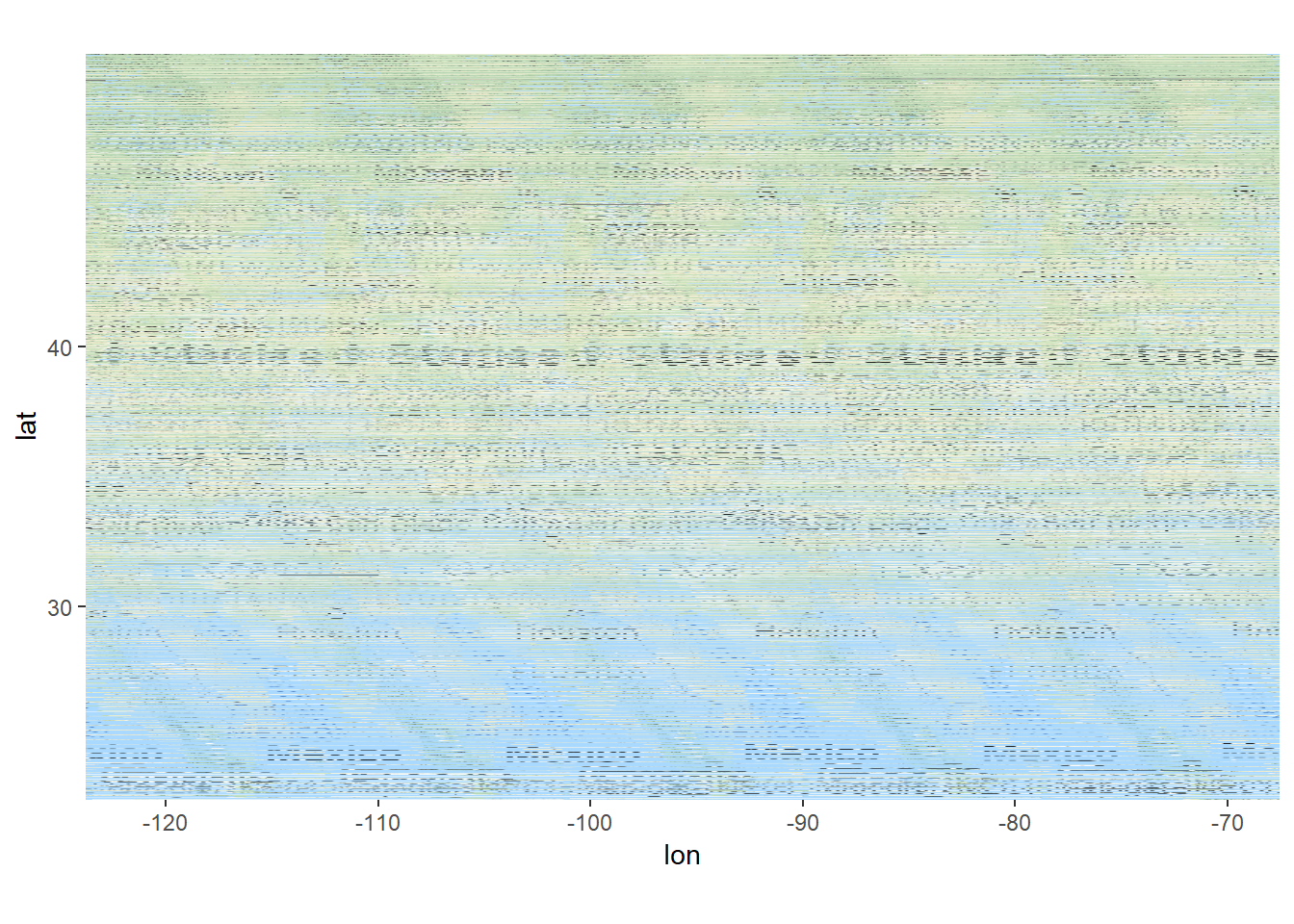

Once we have our map, we can retrieve the coordinates to place our points. Disclaimer - I am working on running this more efficiently, but have been experiencing some issues. ggmap::geocode returns a list of longitude and latitude. For the sake of simplicity, I used the function twice to extract each component. I will update this post with an edit once I figure it out. Advice is welcome!

all_stores_with_coord <- all_stores %>%
  mutate(lon = geocode(address, source = "google")$lon,
         lat = geocode(address, source = "google")$lat)

UPDATE: Turns out there is a mutate_geocode function that will append the lon and lat columns to your dataset!

all_stores_with_coord <- all_stores %>%
  mutate_geocode(address)

This portion of code takes some time, depending on how many queries are ran. This becomes cumbersome if you need to rerun the script for updates to your analysis. To streamline, I wrote the dataframe with coordinates to a local .csv file.

all_stores_with_coord %>% write_csv("stores_with_coords.csv")

Now, for stand alone analysis, the .csv can be read in and runs much faster.

all_stores_with_coord <- read_csv("stores_with_coords.csv")

Now for the finale! ggmap is able to be plugged into a ggplot type pipeline using +. Below, we plot the map, layer on the points corresponding to store locations using our compiled list of stores, scale the color of the points manually, then apply some cleaning of the plot by removing axis lines, titles, and tick marks, and repositiong the legend.

ggmap(mapped_region) +
  geom_point(aes(x = lon, y = lat, col = retailer), alpha = 0.8, data = all_stores_with_coord) +
  scale_color_manual(values = c("blue", "red", "goldenrod")) +
  theme(axis.title = element_blank(),
        axis.text = element_blank(),
        axis.ticks = element_blank(),
        legend.position = "top",
        legend.title = element_blank())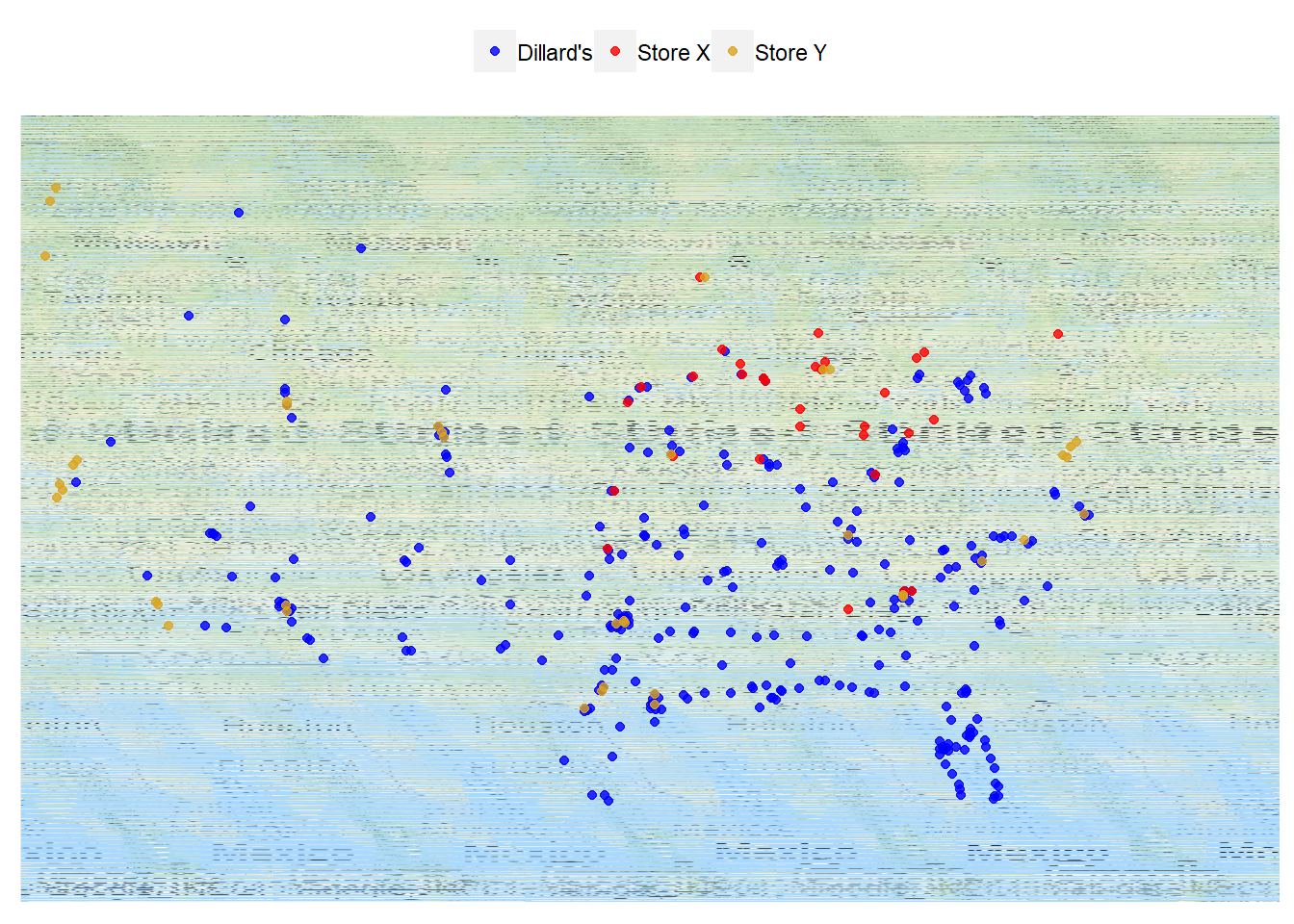

• We can see that Dillard’s has a strong presence in the southern part of the country with some additional, uncontested territory in the Rockies region.
• Store X has more of a hold in the midwest while Store Y is covering the west coast.

Next Steps

We can tell a good amount by eyeballing the above map, but we could do better with more concrete analysis. One idea is to incorporate a distance metric of some sort to find points of high efficiency, defined by distance from the next closest location. With sales data, we could maybe scale the size of the points to line up with volume of business or even highlight places with low penetration of new product launches.