When making updates to your website, it’s hard to know whether or not a change caused an improvement in your KPIs. An A/B Test provides a statistical approach to validate any findings.
I got the opportunity to try out an A/B testing analysis using some fabricated traffic data, along with a hypothesis to check. It’s important to know that there is a ton of front end work to do this right. These experiments needs to be designed, particularly with respect to the sample size needed and effect size.
For this example, I’m lucky enough to have an experiment that was designed and completed before I can access to the data. The practice is focused on the statistical analysis. Check out this account from AirBnB that shows the importance of design and context when tackling these types of problems.
The below covers the presented hypothesis, background information, a full statistical analysis, and next-step suggestions.
Packages
All of the data was in an Excel spreadsheet, so I used readxl to import. For wrangling, I brought in dplyr via the tidyverse package. knitr and kableExtra help for making pretty tables for reports.
knitr::opts_chunk$set(message = FALSE, warning = FALSE)

library(tidyverse)
library(readxl)
library(knitr)
library(kableExtra)
Background - Presented Hypothesis
I believe that presenting the user with large category buttons on the mobile homepage will allow users to more easily navigate to product. If I’m right, we’ll see an increase in product views and downstream metrics including order conversion.
We’ve got data on the control site and 2 variants over a 16 day period.
| Version | Description |
|---|---|
| A | control, standard content slot (no category links) |
| B | smaller horizontal text-based links on a black background, ‘shop by category’ is displayed across the top |
| C | larger vertical text links overlaid on product images in the background |
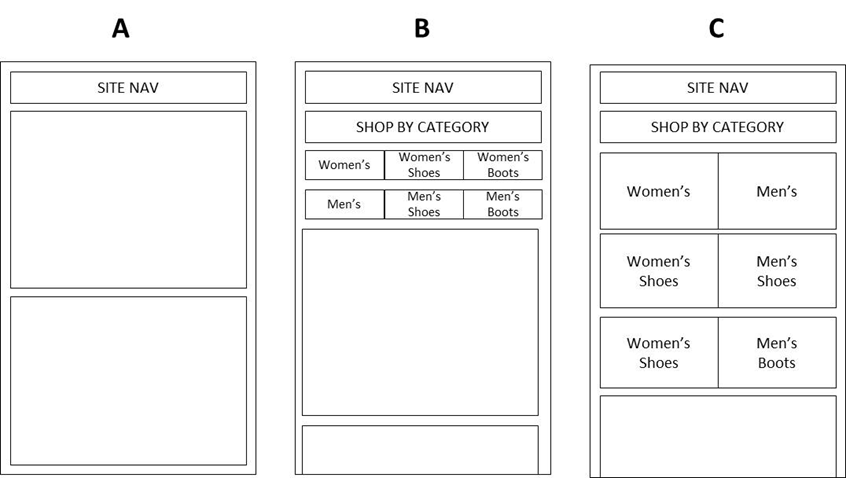
Based on the hypothesis, we can go ahead with an A/B test comparing the control to variant C, since it contains larger buttons. The tested metric will be product viewing rate, or ‘product site visits’ / ‘total home page visits’.
Some additional color on the key metrics recorded:
| Key.Metric | Definition |
|---|---|
| Visits | the number of visits to the site |
| Bounces | a visit who leaves the site without interacting with the page |
| Category_Link_Click_Visits | a visit who clicks a test category link (men’s, women’s, women’s shoe, men’s shoes, women’s boots, men’s boots) |
| Product_View_Visit | a visit who saw a product page |
| Cart_Visit | a visit who saw the cart page |
| Orders | a visit who made a purchase |
| Revenue | sales during the period |
Formal Hypotheses
H0: The product viewing rate is the same for website variants A and C.
Reading in data, extracting KPIs
Getting a look at the table, we see that most of the columns are numeric. When importing, I factored the version variable.
ab_data <- read_excel("AB_test.xlsx", sheet = "key_metrics") %>%
  mutate(Version = factor(Version))

ab_data
## # A tibble: 48 x 9
## Day Version Homepage_Visits Bounces Category_Link_C~ Product_View_Vi~
## <dbl> <fct> <dbl> <dbl> <dbl> <dbl>
## 1 1 A 1260 214 0 652
## 2 2 A 1342 194 0 762
## 3 3 A 1351 204 0 739
## 4 4 A 1323 212 0 668
## 5 5 A 1688 265 0 896
## 6 6 A 1950 277 0 1100
## 7 7 A 1257 222 0 649
## 8 8 A 1239 195 0 645
## 9 9 A 891 146 0 478
## 10 10 A 869 134 0 467
## # ... with 38 more rows, and 3 more variables: Cart_Visits <dbl>,
## # Orders <dbl>, Revenue <dbl>For calculations, the 2 versions were separated, summed, with key conversion metrics calculated, which is the rate of users who entered the website that ended up somewhere down the purchasing funnel.
# Calculate total homepage visits, product views,
# and conversion rate for control and large button variant.
control <- ab_data %>%
  filter(Version == "A") %>%
  summarize(homepage_visits = sum(Homepage_Visits),
            product_view_visits = sum(Product_View_Visit),
            cart_visit = sum(Cart_Visits),
            orders = sum(Orders)) %>%
  mutate(prod_rate = product_view_visits / homepage_visits,
         cart_rate = cart_visit / homepage_visits,
         order_rate = orders / homepage_visits)

variant <- ab_data %>%
  filter(Version == "C") %>%
  summarize(homepage_visits = sum(Homepage_Visits),
            product_view_visits = sum(Product_View_Visit),
            cart_visit = sum(Cart_Visits),
            orders = sum(Orders)) %>%
  mutate(prod_rate = product_view_visits / homepage_visits,
         cart_rate = cart_visit / homepage_visits,
         order_rate = orders / homepage_visits)
Statistic Calculation
The test statistic is the difference between the two conversion rates. Again, we want to see if the change in user experience generated a change in the chance that user makes it to a product page. Note that I have the calculation assignments wrapped in parentheses - doing this assigns your variable and prints it!
(test_stat <- variant$prod_rate - control$prod_rate)## [1] 0.03781852Calculate pooled prop, standard error, z statistic, and p-value. Thanks to rcuevass for the great refresher in the statistics!
(pooled_prop <- (control$product_view_visits + variant$product_view_visits) /
  (control$homepage_visits + variant$homepage_visits))
## [1] 0.5560487(std_err <- sqrt(pooled_prop*(1 - pooled_prop) *
(1/control$homepage_visits + 1/variant$homepage_visits)))## [1] 0.004907679(z_stat <- test_stat/std_err)## [1] 7.705988(p_value <- pnorm(z_stat, lower.tail = FALSE))## [1] 6.491719e-15
Conclusions
The larger buttons produced a 370 basis point lift in the product viewing rate. The calculated p-value satisfies a very stringent alpha level, which lines up with a difference this large. I would recommend adopting the design with large category buttons.
As for downstream metrics, my initial reaction is to build different tests to move the consumer along the conversion funnel. Said differently, what can we do to get the visitor from the product view page to the Product Description Page or the cart? The effect of the category buttons on the end conversion rate is something I’m interested in: does an experience earlier in the order funnel affect the rates a few steps down into the funnel?
However, for completeness, see below similarly calculated p-values for the difference in cart viewing and order conversion rates.
For cart views:
(p_value <- pnorm(z_stat, lower.tail = FALSE))## [1] 0.8487188For orders:
(p_value <- pnorm(z_stat, lower.tail = FALSE))## [1] 0.6132222These larger p-values imply that any difference between the cart viewing and conversion rates for the control and the variant are most likely due to chance.
More Investigations, based on provided data
- Large buttons vs small buttons by using category click links metric.
- Dig into which of the buttons performed stronger - maybe men’s boots had higher click through - why?
- Create a test for more specific category links like “Camp”, “Run”, and “Trail.”